Web Application Development with R Using Shiny - Book review

As may already know (As I have said this a thousand times) I love R -:) And of course...I love Shiny -;)

Today I had the opportunity to read a nice little book called Web Application Development with R using Shiny.

This book starts of course with a small introduction to R, which is more than enough to get started as Shiny will have you coding in no time. Shiny makes it really easy to create web applications using R as its backend.

The explanation of Shiny and its components is pretty well detailed with easy to medium to hard examples...and even when I'm myself a seasoned Shiny developer...there were a lot of things for me to learn...which is always something cool -;)

For example...although I suspect about this...I never tried it and this book just confirm that we can indeed use custom HTML, JavaScript and even JQuery in interaction with Shiny...which for sure open a new way of possibility when developing web applications with R.

Well...let's see a couple of examples shown in the book, so you can get an idea of what Shiny can do...

For sure, a book covering a single package can't be too long...that's why I call this a "nice little book"...but in the end...I'm surprise that the author managed to actually make a book out of it...with examples and lots of code to give us a full overview of Shiny and more than a better starting point to make us start developing our own applications...

If you haven't used R before or you have use it but have never deal with Shiny...this book is totally for you...go ahead and buy it! It's even on sale -;)

Greetings,

Blag.

Calling R from the ERP - A dirty little hack

Since I joined SAP around 2 years ago, I simply stopped using ABAP…even when I use it for almost 11 years when I was a consultant…

A week ago, I was thinking about writing a new blog…something nice…some hacky…something that would allow me to just rest and don’t blog for the rest of the year…

I thought about ERP and R…while some things have been done already like Analytics with SAP and R from Piers Harding. I wanted to actually call R from the ERP instead of the ERP from R -;)

While thinking about this…I thought the best way to do it would be to reuse something that I before on my blog Consuming R from SAP Mobile Platform where I used Rook on Heroku to create a REST page that could be consumable…

So…for this particular blog…I wanted to something simple…call R, generate a graphic and show it on my ABAP program…here’s a small diagram to get things a little bit more clear…

Of course, when I tried this the first time…it failed…miserably…simply because the current implementation of Rook on Heroku doesn't have graphic capabilities on it…so it was impossible to actually generate a graphic…

Let’s get our hands dirty and let’s separate this blogs into steps so it become easier to handle -:)

Compile R with graphic capabilities on Heroku

This step was really a pain…it took me almost a week to get it done…and funny enough the rest of the steps took me about 6 hours…anyway…let’s keep going…

I started by looking at this two awesome projects on Github…rookonheroku and heroku-buildpack-r-build-r I took some chips from both and then create my own script and steps…

If you don’t have Heroku Tool Belt installed…go ahead and grab it…Log into Heroku and do the following…

Steps to install R on Heroku with graphic capabilities
mkdir myproject && cd myproject mkdir bin echo "puts 'OK'" > config.ru echo "source 'http://rubygems.org'\n gem 'rack'" > Gemfile #Open your project folder and modify the Gemfile in Notepad…replace the "\n" by an actual line break. bundle install git init . && git add . && git commit -m "Init" heroku apps:create myproject --stack=cedar git push heroku master #Copy and paste the content of my installR.sh file into your project folder, #also copy the files features.h #and features-orig.h from heroku-buildpack-r-build-r) git add . && git commit -am "message" && git push heroku master heroku ps:scale web=0 heroku run bash cd bin/ ./installR.sh

Here's the code for the installR.sh script...

installR.sh
#!/bin/bash # NOTE: Heroku Cedar Stack # gcc needs to be 4.3 # See http://cran.r-project.org/doc/manuals/R-admin.html for details on building R ## HELPERS function download() { if [ ! -f "$2" ]; then echo Downloading $2... curl $1 -o $2 else echo Got $2... fi } function build() { echo ---------------------------------------------------------------------- echo Building $@... echo ---------------------------------------------------------------------- echo pushd $1 ./configure --prefix=$vendordir/$2 ${@:3} && make && make install && make clean popd > /dev/null echo echo # add to libraries and pkg-config export LD_LIBRARY_PATH="$vendordir/$2:$LD_LIBRARY_PATH" export PKG_CONFIG_PATH="$vendordir/$2/lib/pkgconfig:$PKG_CONFIG_PATH" } ## SCRIPT set -e r_version="${1:-2.13.1}" r_version_major=${r_version:0:1} if [ -z "$r_version" ]; then echo "USAGE: $0 VERSION" exit 1 fi basedir="$( cd -P "$( dirname "$0" )" && pwd )" # create output directory vendordir=/app/vendor mkdir -p $vendordir echo ====================================================================== echo Downloading and unpacking dependancies... echo ====================================================================== # We need to install xz to be able to unzip the gcc package we're going to download in a minute curl http://gfortran.com/download/x86_64/xz.tar.gz -o xz.tar.gz tar xzvf xz.tar.gz # Get and unpack gcc-4.3 binary, including gfortran curl http://gfortran.com/download/x86_64/snapshots/gcc-4.3.tar.xz  -o gcc-4.3.tar.xz ./usr/bin/unxz gcc-4.3.tar.xz tar xvf gcc-4.3.tar # http://www.freetype.org/freetype2/ freetype_version=2.5.0 download http://www.mirrorservice.org/sites/download.savannah.gnu.org/releases/freetype/freetype-$freetype_version.tar.gz  freetype-$freetype_version.tar.gz tar xzf freetype-$freetype_version.tar.gz # http://directfb.org/ directfb_version=1.2.9 directfb_ver_major=${directfb_version:0:3} download http://directfb.org/downloads/Core/DirectFB-$directfb_ver_major/DirectFB-$directfb_version.tar.gz  DirectFB-$directfb_version.tar.gz tar xzf DirectFB-$directfb_version.tar.gz # http://www.libpng.org/pub/png/libpng.html libpng_version=1.2.50 download ftp://ftp.simplesystems.org/pub/libpng/png/src/libpng12/libpng-$libpng_version.tar.gz  libpng-$libpng_version.tar.gz tar xzf libpng-$libpng_version.tar.gz # http://www.cairographics.org pixman_version=0.29.4 download http://www.cairographics.org/snapshots/pixman-$pixman_version.tar.gz  pixman-$pixman_version.tar.gz tar xzf $basedir/pixman-$pixman_version.tar.gz # http://www.freedesktop.org/software/fontconfig fontconfig_version=2.9.0 download http://www.freedesktop.org/software/fontconfig/release/fontconfig-$fontconfig_version.tar.gz  fontconfig-$fontconfig_version.tar.gz tar xzf $basedir/fontconfig-$fontconfig_version.tar.gz # http://www.cairographics.org cairo_version=1.9.14 download http://www.cairographics.org/snapshots/cairo-$cairo_version.tar.gz  cairo-$cairo_version.tar.gz tar xzf $basedir/cairo-$cairo_version.tar.gz # http://www.pango.org #pango_ver=1.35 #pango_version=$pango_ver.0 #download http://ftp.gnome.org/pub/GNOME/sources/pango/$pango_ver/pango-$pango_version.tar.xz  #pango-$pango_version.tar.xz #tar xJf $basedir/pango-$pango_version.tar.xz # R download http://cran.r-project.org/src/base/R-$r_version_major/R-$r_version.tar.gz  R-$r_version.tar.gz tar xzf R-$r_version.tar.gz # http://gcc.gnu.org/wiki/GFortran gcc_version=4.3 download http://gfortran.com/download/x86_64/snapshots/gcc-$gcc_version.tar.xz  gcc-$gcc_version.tar.xz tar xJf $basedir/gcc-$gcc_version.tar.xz -C $vendordir # patch gcc features.h file # see http://permalink.gmane.org/gmane.comp.gcc.help/40166 mkdir -p $vendordir/gcc-$gcc_version/lib/gcc/x86_64-unknown-linux-gnu/$gcc_version/include-fixed cp $basedir/features.h $vendordir/gcc-$gcc_version/lib/gcc/x86_64-unknown-linux-gnu/$gcc_version/include-fixed/features.h # https://www.gnu.org/software/libc/ glibc_version=2.7 glibc_version_x=2.7ds1 download ftp://ftp.gunadarma.ac.id/linux/debian/pool/main/g/glibc/glibc_2.7.orig.tar.gz  glibc_$glibc_version.tar.gz tar xzf $basedir/glibc_$glibc_version.tar.gz -C $vendordir tar xjf $vendordir/glibc-$glibc_version/glibc-$glibc_version_x.tar.bz2 -C $vendordir echo ============================================================ echo Building dependencies... echo ====================================================================== build "$basedir/freetype-$freetype_version" freetype build "$basedir/DirectFB-$directfb_version" DirectFB build "$basedir/libpng-$libpng_version" libpng build "$basedir/pixman-$pixman_version" pixman build "$basedir/fontconfig-$fontconfig_version" fontconfig build "$basedir/cairo-$cairo_version" cairo # copy over missing header files cp $basedir/cairo-$cairo_version/src/*.h $vendordir/cairo/include #build $basedir/pango-$pango_version pango # build R echo ============================================================ echo Building R echo ============================================================ cd $basedir/R-$r_version/ export LDFLAGS="-L$vendordir/gcc-$gcc_version/lib64" export CPPFLAGS="-I$vendordir/glibc-$glibc_version/string/ -I$vendordir/glibc-$glibc_version/time" export PATH="$vendordir/gcc-$gcc_version/bin:$PATH" echo ---------------------------------------------------------------------- echo LD_LIBRARY_PATH=$LD_LIBRARY_PATH echo PKG_CONFIG_PATH=$PKG_CONFIG_PATH echo ---------------------------------------------------------------------- ./configure --prefix=$vendordir/R --enable-R-shlib --with-readline=no --with-x=yes make cd /app/bin #ln -s R-2.15-1/bin/R ln -s R-2.13.1/bin/R rm gcc-4.3.tar rm glibc_2.7.orig.tar.gz rm R.tar.gz rm xz.tar.gz rm -rf usr/ rm -rf gcc-4.3/bin rm -rf gcc-4.3/lib rm -rf gcc-4.3/libexec rm -rf gcc-4.3/info rm -rf gcc-4.3/man rm -rf gcc-4.3/share rm -rf gcc-4.3/include rm glibc-2.7/*.tar.bz cd bin/glibc-2.7/ rm -rf abilist/ abi-tags aclocal.m4 argp assert/ b* BUGS C* c* d* e* F* g* h* i* I* l* m* M* N* aout/  rm -rf LICENSES n* o* p* P* R* r* scripts/ setjmp/ shadow/ shlib-versions signal/ socket/ soft-fp/  rm -rf stdio-common/ stdlib/ streams/ sunrpc/ sysdeps/ sysvipc/ termios/ test-skeleton.c timezone  rm -rf tls.make.c version.h Versions.def wcsmbs/ wctype/ WUR-REPORT cd ../R-2.13.1 rm -rf src rm Make* rm -rf doc rm NEWS* rm -rf test rm config* rm O* README ChangeLog COPYING INSTALL SVN-REVISION VERSION NEED etc

With that…you will have a full R installation with graphic capabilities…of course…you will need to delete all the garbage generated…but we will get there later…

Now…we need to install Rook…but we need version 1.0-2 so we need to download it and install it from the source…

Download Rook 1.0-2
Wget http://cran.r-project.org/src/contrib/Archive/Rook/Rook_1.0-2.tar.gz -o Rook_1.0-2.tar.gz

Then launch R…simply call it by saying…

Calling R
R

As it will launch the R environment…

Installing Rook
install.packages(/Rook_1.0-2.tar.gz, repos = NULL, type="source") #Now we can simply quit R q()

As I was lazy to work more on the script to delete those files automatically…basically…the “bin” folder should look like this…

And the “vendor” folder like this…

Please remove the folders by using…

Removing folders
rm –rf name_of_folder

Once we’re done…we need to pack our stuff and sent it somewhere else, as Heroku is read only…once we log off…we lost everything…

Backup your work
tar -cvzf bin.tar.gz bin tar -cvzf vendor.tar.gz vendor scp bin.tar.gz me@myserver.com:/myproject/bin.tar.gz scp vendor.tar.gz me@myserver.com:/myproject/vendor.tar.gz #For scp you actually need a server…and I had my R on AWS…so I did used that…it might look like this… scp -i XXX_X.pem bin.tar.gz root@XX.XX.XXX.XXX:/Blag/bin.tar.gz

Once we have everything saved…we can close the Heroku session and keep going…we can use WinSCP to copy our packed folders from our AWS server into our local project folder…uncompressed them and copy the following files from rookonheroku…

• config.ru
• demo.R
• Procfile

Then…you can simply send everything back to Heroku…

Last push on Heroku
git add . && git commit -am "message" && git push heroku master heroku ps:scale web=1

Of course…this is a lot of work…and I mean it…lot

So…I have upload the final compiled version to GitHub -;) To get it…simply do this…

Getting Blagrook
git clone git:// github.com/atejada/BlagRook.git yourproject  #(This will clone my Github and create a folder called yourproject to store the codes) heroku create myapp #(Create an application for the Rook script) git push heroku master #(This allows to pass everything from my yourproject folder to your Heroku account)

Create the code for the Rook application

On last thing we need to do…is to create the Rook application that it’s going to work on our Rook server…

demo.R
library(Rook) newapp<-function(env){ req<-Rook::Request$new(env) res<-Rook::Response$new() carrid_param<-c(req$params()$carrid) seats_param<-c(req$params()$seats) carrid_param<-strsplit(carrid_param,",") carrid_param<-c(carrid_param[[1]][1],carrid_param[[1]][2], carrid_param[[1]][3]) seats_param<-strsplit(seats_param,",") seats_param<-c(as.numeric(seats_param[[1]][1]),as.numeric(seats_param[[1]][2]), as.numeric(seats_param[[1]][3])) params<-data.frame(carrid_param,seats_param) bmp("R_Plot.bmp",type=c("cairo")) dotchart(params$seats_param,labels=params$carrid_param, xlab="Number of seats",ylab="Carriers") dev.off() to.read = file("R_Plot.bmp", "rb") x<-readBin(to.read, raw(),n=231488) hex<-paste(x, collapse = "") res$write(hex) res$finish() } server = Rhttpd$new() server$add(app = newapp, name = "summarize") server$start(listen="0.0.0.0", port=as.numeric(Sys.getenv("PORT"))) while(T) { Sys.sleep(10000) }

In a few words what is happening here is simple...we receive the parameters "carrid" and "seats"...both came as a string with "," so we use strsplit to separate them and then create a factor with the values. In the case of "seats" we need it to be numeric so we use the as.numeric function. Finally we create a data.frame combining "carrid" and "seats". Using "Cairo" (That's why we needed graphic capabilities on R) we create a Bitmap file which is going to be the result of creating a dotchart. Once it has been created, we read it, using the readBin function we get it's Hexadecimal representation. Using the function paste and its collapse method, we put everything on a big string and send it back...easy as pie -;)

I’m sure that you will wonder how I came out with the number 231488 on the readBin line…well…I download a nice Hexadecimal Editor called HxD then I create the graphic on my local R and load it…the I went to the last line and took the Hex number…

Using the calculator I simply changed the Hex value 38830 to decimal, multiply it by 16 and then add 16 more as the first line doesn’t count…simply and easy -;)

Create the function module ZUPLOAD_GRAPHICS_TABLE

This function module will allow us to upload the generated graphic into SE78.

ZUPLOAD_GRAPHICS_TABLE
FUNCTION ZUPLOAD_GRAPHICS_TABLE. *"---------------------------------------------------------------------- *"*"Local Interface: *" IMPORTING *" REFERENCE(OBJECT) TYPE TDOBJECT DEFAULT 'GRAPHICS' *" REFERENCE(NAME) TYPE TDOBNAME *" REFERENCE(BTYPE) TYPE TDBTYPE *" REFERENCE(ID) TYPE TDID DEFAULT 'BMAP' *" REFERENCE(RESOLUTION) TYPE TDRESIDENT OPTIONAL *" REFERENCE(RESIDENT) TYPE TDRESIDENT OPTIONAL *" REFERENCE(AUTOHEIGHT) TYPE TDAUTOHGHT OPTIONAL *" TABLES *" T_BITMAP OPTIONAL *"---------------------------------------------------------------------- TYPES: TY_BOOLEAN(1) TYPE C. TYPES: BEGIN OF TY_SBDST_CONTENT. INCLUDE STRUCTURE BAPICONTEN. TYPES: END OF TY_SBDST_CONTENT. TYPES: SBDST_COMPONENTS LIKE BAPICOMPON OCCURS 1, SBDST_PROPERTIES LIKE BAPIPROPER OCCURS 1, SBDST_SIGNATURE LIKE BAPISIGNAT OCCURS 1, SBDST_CONTENT LIKE BAPICONTEN OCCURS 1. DATA: T_BDS_CONTENT TYPE STANDARD TABLE OF TY_SBDST_CONTENT, WA_BDS_COMPONENTS TYPE LINE OF SBDST_COMPONENTS, L_BDS_PROPERTIES TYPE SBDST_PROPERTIES, L_BDS_COMPONENTS TYPE SBDST_COMPONENTS, T_STXBITMAPS TYPE STANDARD TABLE OF STXBITMAPS WITH HEADER LINE, WA_BDS_SIGNATURE TYPE LINE OF SBDST_SIGNATURE, L_BDS_SIGNATURE TYPE SBDST_SIGNATURE, L_BDS_CONTENT TYPE SBDST_CONTENT, WA_STXBITMAPS TYPE STXBITMAPS, WA_BDS_PROPERTIES TYPE LINE OF SBDST_PROPERTIES. DATA: W_BYTECOUNT TYPE I, W_COLOR(1) TYPE C, W_WIDTH_TW TYPE STXBITMAPS-WIDTHTW, W_HEIGHT_TW TYPE STXBITMAPS-HEIGHTTW, W_WIDTH_PIX TYPE STXBITMAPS-WIDTHPIX, W_HEIGHT_PIX TYPE STXBITMAPS-HEIGHTPIX, W_RESOLUTION TYPE STXBITMAPS-RESOLUTION, W_BDS_BYTECOUNT TYPE I, W_TYPE TYPE STXBITMAPS-TDBTYPE, W_DOCID TYPE STXBITMAPS-DOCID. DATA: L_BDS_OBJECT TYPE REF TO CL_BDS_DOCUMENT_SET. CONSTANTS: C_TRUE TYPE TY_BOOLEAN VALUE 'X', C_FALSE TYPE TY_BOOLEAN VALUE SPACE, C_BDS_MIMETYPE TYPE BDS_MIMETP VALUE 'application/octet-stream', C_BDS_CLASSNAME TYPE SBDST_CLASSNAME VALUE 'DEVC_STXD_BITMAP', C_BDS_CLASSTYPE TYPE SBDST_CLASSTYPE VALUE 'OT'. IF BTYPE = 'BMON'. W_COLOR = C_FALSE. ELSE. W_COLOR = C_TRUE. ENDIF. CALL FUNCTION 'SAPSCRIPT_CONVERT_BITMAP_BDS' EXPORTING COLOR = W_COLOR FORMAT = 'BMP' BITMAP_BYTECOUNT = W_BYTECOUNT compress_bitmap = 'X' IMPORTING WIDTH_TW = W_WIDTH_TW HEIGHT_TW = W_HEIGHT_TW WIDTH_PIX = W_WIDTH_PIX HEIGHT_PIX = W_HEIGHT_PIX DPI = W_RESOLUTION BDS_BYTECOUNT = W_BDS_BYTECOUNT TABLES BITMAP_FILE = T_BITMAP BITMAP_FILE_BDS = T_BDS_CONTENT EXCEPTIONS FORMAT_NOT_SUPPORTED = 1 NO_BMP_FILE = 2 BMPERR_INVALID_FORMAT = 3 BMPERR_NO_COLORTABLE = 4 BMPERR_UNSUP_COMPRESSION = 5 BMPERR_CORRUPT_RLE_DATA = 6 OTHERS = 7. CREATE OBJECT L_BDS_OBJECT. WA_BDS_COMPONENTS-DOC_COUNT = '1'. WA_BDS_COMPONENTS-COMP_COUNT = '1'. WA_BDS_COMPONENTS-MIMETYPE = C_BDS_MIMETYPE. WA_BDS_COMPONENTS-COMP_SIZE = W_BYTECOUNT. APPEND WA_BDS_COMPONENTS TO L_BDS_COMPONENTS. W_TYPE = 'BSD'. SELECT SINGLE * INTO T_STXBITMAPS FROM STXBITMAPS WHERE TDOBJECT = OBJECT AND TDNAME = NAME AND TDID = ID AND TDBTYPE = BTYPE. IF SY-SUBRC = 0. READ TABLE T_STXBITMAPS INDEX 1. W_DOCID = T_STXBITMAPS-DOCID. ELSE. CLEAR W_DOCID. ENDIF. IF W_DOCID IS INITIAL. WA_BDS_SIGNATURE-DOC_COUNT = '1'. APPEND WA_BDS_SIGNATURE TO L_BDS_SIGNATURE. CALL METHOD L_BDS_OBJECT->CREATE_WITH_TABLE EXPORTING CLASSNAME = C_BDS_CLASSNAME CLASSTYPE = C_BDS_CLASSTYPE COMPONENTS = L_BDS_COMPONENTS CONTENT = T_BDS_CONTENT CHANGING SIGNATURE = L_BDS_SIGNATURE EXCEPTIONS OTHERS = 1. READ TABLE L_BDS_SIGNATURE INDEX 1 INTO WA_BDS_SIGNATURE TRANSPORTING DOC_ID. IF SY-SUBRC = 0. W_DOCID = WA_BDS_SIGNATURE-DOC_ID. ENDIF. ELSE. CALL METHOD L_BDS_OBJECT->UPDATE_WITH_TABLE EXPORTING CLASSNAME = C_BDS_CLASSNAME CLASSTYPE = C_BDS_CLASSTYPE DOC_ID = W_DOCID DOC_VER_NO = '1' DOC_VAR_ID = '1' CHANGING COMPONENTS = L_BDS_COMPONENTS CONTENT = T_BDS_CONTENT EXCEPTIONS NOTHING_FOUND = 1 OTHERS = 2. ENDIF. WA_STXBITMAPS-TDNAME = NAME. WA_STXBITMAPS-TDOBJECT = OBJECT. WA_STXBITMAPS-TDID = ID. WA_STXBITMAPS-TDBTYPE = BTYPE. WA_STXBITMAPS-DOCID = W_DOCID. WA_STXBITMAPS-WIDTHPIX = W_WIDTH_PIX. WA_STXBITMAPS-HEIGHTPIX = W_HEIGHT_PIX. WA_STXBITMAPS-WIDTHTW = W_WIDTH_TW. WA_STXBITMAPS-HEIGHTTW = W_HEIGHT_TW. WA_STXBITMAPS-RESOLUTION = RESOLUTION. WA_STXBITMAPS-RESIDENT = RESIDENT. WA_STXBITMAPS-AUTOHEIGHT = AUTOHEIGHT. WA_STXBITMAPS-BMCOMP = 'X'. INSERT INTO STXBITMAPS VALUES WA_STXBITMAPS. ENDFUNCTION.

Create the ABAP program to make it all happen…

ZROOK
*&--------------------------------------------------------------------&* *& Report ZROOK &* *&--------------------------------------------------------------------&* *& Author: Alvaro "Blag" Tejada Galindo &* *& Company: SAP Labs Palo Alto &* *& Date: November 11, 2013 &* *& Modified on: November 18, 2013 &* *& Reason: Finish the code -;) &* *&********************************************************************&* REPORT ZROOK NO STANDARD PAGE HEADING. TYPES : BEGIN OF ty_bitmap, l(64) TYPE x, END OF ty_bitmap. TYPES: BEGIN OF TY_GRAPHIC_TABLE, LINE(255) TYPE X, END OF TY_GRAPHIC_TABLE. types: begin of ty_flights, carrid type sflight-carrid, seatsocc type sflights-seatsocc, end of ty_flights. DATA: it_bitmap TYPE STANDARD TABLE OF ty_bitmap, i_po_data TYPE STANDARD TABLE OF string, i_bitmap TYPE STANDARD TABLE OF string, T_GRAPHIC_TABLE TYPE STANDARD TABLE OF TY_GRAPHIC_TABLE, t_flights type STANDARD TABLE OF ty_flights, bitmap type string, client TYPE REF TO if_http_client, container TYPE REF TO cl_gui_custom_container, lv_length TYPE i, lv_content TYPE xstring, lr_mime_rep TYPE REF TO if_mr_api, OUTXSTRING type xstring, URL(255) TYPE C, PICTURE TYPE REF TO CL_GUI_PICTURE, L_BYTECOUNT TYPE I, L_CONTENT TYPE STANDARD TABLE OF BAPICONTEN, GRAPHIC_SIZE TYPE I, bin TYPE xstring, conv TYPE REF TO cl_abap_conv_in_ce, response TYPE string, carrid type string, seats type string, seatsocc type string, param type string. FIELD-SYMBOLS: <fs_bitmap> like line of i_bitmap, <fs_itbitmap> like line of it_bitmap, <fs_po_data> like line of i_po_data, <fs_flight> like line of t_flights. START-OF-SELECTION. perform get_data. perform call_rook. perform create_graphic. perform show_graphic. *&---------------------------------------------------------------------* *& Form GET_DATA *&---------------------------------------------------------------------* FORM GET_DATA. select carrid sum( seatsocc ) into table t_flights from sflights group by carrid. loop at t_flights ASSIGNING <fs_flight>. seatsocc = <fs_flight>-seatsocc. CONDENSE seatsocc NO-GAPS. CONCATENATE carrid <fs_flight>-carrid into carrid SEPARATED BY ','. CONCATENATE seats seatsocc into seats SEPARATED BY ','. ENDLOOP. replace regex '\A,' in carrid with space. replace regex '\A,' in seats with space. CONCATENATE '/custom/summarize?carrid=''' carrid '''&seats=' seats into param. ENDFORM. " GET_DATA *&---------------------------------------------------------------------* *& Form CALL_ROOK *&---------------------------------------------------------------------* FORM CALL_ROOK. CALL METHOD cl_http_client=>create EXPORTING host = 'blagrook.herokuapp.com' scheme = 1 IMPORTING client = client. client->request->set_method( if_http_request=>co_request_method_get ). cl_http_utility=>set_request_uri( request = client->request uri = param ). client->send( ). client->receive( ). bin = client->response->get_data( ). conv = cl_abap_conv_in_ce=>create( input = bin ). conv->read( IMPORTING data = response ). client->close( ). ENDFORM. " CALL_ROOK *&---------------------------------------------------------------------* *& Form CREATE_GRAPHIC *&---------------------------------------------------------------------* FORM CREATE_GRAPHIC. bitmap = response. TRANSLATE bitmap TO UPPER CASE. CALL FUNCTION 'SOTR_SERV_STRING_TO_TABLE' EXPORTING TEXT = bitmap LINE_LENGTH = 128 TABLES TEXT_TAB = i_bitmap. loop at i_bitmap ASSIGNING <fs_bitmap>. APPEND INITIAL LINE TO it_bitmap ASSIGNING <fs_itbitmap>. <fs_itbitmap>-l = <fs_bitmap>. ENDLOOP. CALL FUNCTION 'ZUPLOAD_GRAPHICS_TABLE' EXPORTING OBJECT = 'GRAPHICS' NAME = 'BLAG' BTYPE = 'BMON' ID = 'BMAP' TABLES T_BITMAP = it_bitmap. ENDFORM. " CREATE_GRAPHIC *&---------------------------------------------------------------------* *& Form SHOW_GRAPHIC *&---------------------------------------------------------------------* FORM SHOW_GRAPHIC. CALL FUNCTION 'SAPSCRIPT_GET_GRAPHIC_BDS' EXPORTING I_OBJECT = 'GRAPHICS' I_NAME = 'BLAG' I_ID = 'BMAP' I_BTYPE = 'BMON' IMPORTING E_BYTECOUNT = L_BYTECOUNT TABLES CONTENT = L_CONTENT EXCEPTIONS NOT_FOUND = 1 BDS_GET_FAILED = 2 BDS_NO_CONTENT = 3 OTHERS = 4. CALL FUNCTION 'SAPSCRIPT_CONVERT_BITMAP' EXPORTING OLD_FORMAT = 'BDS' NEW_FORMAT = 'BMP' BITMAP_FILE_BYTECOUNT_IN = L_BYTECOUNT IMPORTING BITMAP_FILE_BYTECOUNT = GRAPHIC_SIZE TABLES BDS_BITMAP_FILE = L_CONTENT BITMAP_FILE = T_GRAPHIC_TABLE EXCEPTIONS OTHERS = 1. CALL FUNCTION 'DP_CREATE_URL' EXPORTING TYPE = 'IMAGE' SUBTYPE = 'BMP' TABLES DATA = T_GRAPHIC_TABLE CHANGING URL = URL. CREATE OBJECT container EXPORTING container_name = '' repid = 'SAPMSSY0' dynnr = '0120'. container->set_top( -85 ). container->set_left( 120 ). container->set_width( 580 ). container->set_height( 580 ). CREATE OBJECT PICTURE EXPORTING PARENT = container. CALL METHOD PICTURE->LOAD_PICTURE_FROM_URL EXPORTING URL = URL. CALL METHOD PICTURE->SET_DISPLAY_MODE EXPORTING DISPLAY_MODE = PICTURE->DISPLAY_MODE_FIT_CENTER. WRITE ''. ENDFORM. " SHOW_GRAPHIC

When we run our program…we will call our Rook application on Heroku, which will receive the sum of seats for three carriers and then create a graphic, read it’s hexadecimal representation, give back to ABAP which will in turn create it on SE78 and then read it to show it on screen…now…you will not get the best resolution ever…and will assume it’s because “Cairo” doesn’t really support bmp files, or because the graphic is getting transported and changed all the way…so…it doesn't look good…but heck! We’re calling R from the ERP…what else do you want? -:D

It was really fun…so see you next year -;)

Greetings,

Blag.

Developer Experience.

Columbus Day on Packt Publishing!

Get a 50% discount on Packt Publishing books http://bit.ly/1bqvB29  #COL50

Greetings,

Blag.
Developer Experience.

SAP HANA - Let's talk about Rows and Columns

As we all know...SAP HANA can handle table creation in two ways...Rows and Columns. Row tables are suppose to be better for tables that get updated very often and Column tables for tables that doesn't get updated very often...Column Tables are supposed to be faster when it comes to read their contents.

As I have never actually test this...I create two Python scripts to generate 1 million records for two tables...DOC_HEADER and DOC_DETAILS. These two tables share the DOCUMENT_ID, YEAR and AREA but as the information get created randomly, chances that both tables have some values in common are not really known...

For the sake of the example I create both tables DOC_HEADER and DOC_DETAILS using both Rows and Column types and build another Python script to measure the reading time...

Column_Row_SAPHANA_Test.py
import dbapi import time conn = dbapi.connect('*****', 30015, 'SYSTEM', '****') cur = conn.cursor() query = '''SELECT H."DOCUMENT_ID", H."YEAR", H."AREA", SUM("AMOUNT") AS AMOUNT FROM "BLAG"."DOC_HEADER_ROW" AS H INNER JOIN "BLAG"."DOC_DETAIL_ROW" AS D ON H."DOCUMENT_ID" = D."DOCUMENT_ID" AND H."YEAR" = D."YEAR" AND H."AREA" = D."AREA" GROUP BY H."DOCUMENT_ID", H."YEAR", H."AREA"''' start = time.clock() cur.execute(query) ret = cur.fetchall() end = time.clock() counter = 0 for row in ret: counter += 1 time_taken = end - start print("Row Store - %s records in %s seconds") %(counter, time_taken) query = '''SELECT H."DOCUMENT_ID", H."YEAR", H."AREA", SUM("AMOUNT") AS AMOUNT FROM "BLAG"."DOC_HEADER_COLUMN" AS H INNER JOIN "BLAG"."DOC_DETAIL_COLUMN" AS D ON H."DOCUMENT_ID" = D."DOCUMENT_ID" AND H."YEAR" = D."YEAR" AND H."AREA" = D."AREA" GROUP BY H."DOCUMENT_ID", H."YEAR", H."AREA"''' start = time.clock() cur.execute(query) ret = cur.fetchall() end = time.clock() counter = 0 for row in ret: counter += 1 time_taken = end - start print("Column Store - %s records in %s seconds") %(counter, time_taken)

Both queries do the exact same thing...they do an INNER JOIN between the two tables...using ROW store for the first one and COLUMN store for the second one...

Let's run this 3 times and see what happens -;)

Benchmark
Row Store - 7669 records in 2.45972177882 seconds Column Store - 7669 records in 1.59409638594 seconds Row Store - 7669 records in 2.32650395252 seconds Column Store - 7669 records in 1.68382533783 seconds Row Store - 7669 records in 2.44930342075 seconds Column Store - 7669 records in 1.52396673192 seconds

As we can see...we have a constant gain of about 38% faster when using Column store...

Greetings,

Blag.
Developer Experience.

Software Development on the SAP HANA Platform - Book review

Some time ago I did a technical review for SAP HANA Starter from Mark Walker.

This time I had the pleasure to read Software Development on the SAP HANA Platform a really nice book for beginners on SAP HANA.

The book is really good and full of pictures, examples and clear explanation that will get from an SAP HANA noob to a well versed SAP HANA enthusiast.

Mark cover everything from a single but powerful comparison between SAP HANA and MySQL to XS Development passing of course between the creation of Attribute Views and data provisioning on SAP HANA.

The full book is around 303 pages so you will get what you pay for...a comprehensive guide and tour through the amazing wold of SAP HANA.

So...if you still haven't get your hands dirty with these awesome SAP In-Memory technology, don't waste more time and get the book, you don't be disappointed.

And truth to be said...with the rapid and mass adoption of SAP HANA, many people just want to jump on the wagon and make some money by selling books without real content...Mark Walker does an awesome job of delivering a great learning experience...just in the way I would do it myself...clear examples full of images so you can know exactly what to expect and know exactly what to do next.

Greetings,

Blag.
Developer Experience.

Running R inside SAP HANA Studio

*DANGER* This is just a silly blog and shouldn't be taken any seriously.*DANGER*

Ok...you may wonder...why is Blag writing a silly blog? Well...I'm a Developer Evangelist...and it's my job to keep developers entertained  Also...I have so free time to spare

As you all may know...SAP HANA Studio runs on top of Eclipse...which means that if we can run R on Eclipse...then we can obviously run R on SAP HANA Studio...that's exactly what we're going to do

As easy as it gets...follows this instructions...

• Go to Help --> Install New Software
• Put the following repository

• Choose Walware - StatET

• Once installed, your SAP HANA Studio will restart and you will need to configure R.
• Go to Windows --> Preferences.
• StatET --> Run/Debug --> R Environments --> Add (In my picture, I'm using Edit as I already add it).

• Either on the Command Line or in RStudio, install the following...
• install.packages(c("rj", "rj.gd"), repos="http://download.walware.de/rj-1.1")
• Also install RJava as well...install.packages("RJava")

 Now...you need to start the R console...so...

• Go to the little Green Arrow button and press "R_Console".

Once that it's done, we can go ahead and create our R script...

• Go to File --> New Project --> R Project.
• On the created R Project, right click and select New --> R Script File.

Copy this code inside your new file...

R_from_SAP_HANA.sql
result<-read.table('clipboard',header=TRUE,sep=';') result<-subset(result, !duplicated(DISTANCE)) flights<-data.frame(DISTANCE=as.numeric(result$DISTANCE)) row.names(flights)<-result$FLIGHT d<-dist(as.matrix(flights)) hc<-hclust(d) plot(hc)

Now...go to the "Modeler" perspective...open a SQL Console and write the following...

SAP_HANA_Select.sql
SELECT DISTINCT CITYFROM || '/' || CITYTO "FLIGHT", DISTANCE FROM SFLIGHT.SPFLI WHERE DISTANCE > 0 AND CARRID = 'SQ'

Run it...and here's come the funny part...go to the Result tab and select all records...then press Copy Rows, so the selection gets copied into the Clipboard.

Go back to the StatET perspective and click the "Run file in R via command" button...

When you run the code...you're not going to see any response, unless there's an error...so just go to the R Graphics tab which is at the bottom where the Console window seats...expand it...and you will see a Cluster Dendogram graphic generated -;)

I told you...this was a very silly post...but at least...we never left the SAP HANA Studio -:P

See you next time!

Blag.

Developer Experience.

Forecasting with Neural Network (using SAP HANA and R)

Usually...when I use R...I try to use it with SAP HANA as well...and the most simple way to make them work is for sure an ODBC connection....fast and simple...

First, I went to my SAP HANA Studio to get the query...which is basically...get all the seats (First, Business, Economy) from all flights that happened between 2010 and 2012.

Query from HANA Studio
SELECT FLDATE, SEATSOCC, SEATSOCC_B, SEATSOCC_F FROM SFLIGHT.SFLIGHT WHERE YEAR(FLDATE) BETWEEN '2010' AND '2012'

The result will look like this...

But...we want to have all seats summed up in one variable and also organized by month/year. And while we can do that using SQL...that will take away the fun from R...

Getting and formatting data
library("RODBC") format_date<-function(p_date){ p_date<-as.Date(as.character(p_date),"%Y%m%d") p_date<-format(p_date,"%Y%m") return(p_date) } ch<-odbcConnect("HANA",uid="SYSTEM",pwd="********") result<-sqlQuery(ch,"SELECT FLDATE, SEATSOCC, SEATSOCC_B, SEATSOCC_F FROM SFLIGHT.SFLIGHT WHERE YEAR(FLDATE) BETWEEN '2010' AND '2012'") odbcCloseAll() dates<-result$FLDATE dates<-format_date(dates) result$FLDATE = dates result_agg<-aggregate(cbind(SEATSOCC,SEATSOCC_B,SEATSOCC_F)~.,data=result,FUN=sum) result_total<-data.frame(FLDATE=result_agg$FLDATE,SEATS=result_agg$SEATSOCC+ result_agg$SEATSOCC_B+result_agg$SEATSOCC_F,stringsAsFactors=FALSE)

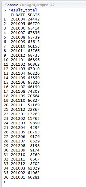
First, by using the RODBC library we connect to our SAP HANA Server. Then, we grab the dates and using a custom function, convert them to Month/Year. We do an aggregation to get the sum of all seats and then built a data frame to hold the data.

When we print out the final result...we will realize something that for sure, escaped our eyes before...

For 2010, the months start on April, meaning that from January to March there's no information...and the same happens to 2012 where the information end on April and from June to December there's nothing.

As we want to do a Forecasting using Neural Network...this incomplete data is never going to work...so we need to do something to fix it...

One thing to do at least for 2012, it's the Moving Average...which is basically grab the values from January to April, sum them, divide them by the number of months and then assign this value to May (201205)...then...grab the value from February to May and do the same thing for June...and so on -:)

For 2010 seems look a little bit more complicated...but it's almost the same...I used something that I like to call Backward Average...despite what the real name is -:P Basically, we grab the values from December to April, sum them, divide the value by the number of months and determine the value for March...and so on...

Let's see the code...

Moving and Backward Average
library("RODBC") format_date<-function(p_date){ p_date<-as.Date(as.character(p_date),"%Y%m%d") p_date<-format(p_date,"%Y%m") return(p_date) } moving_average<-function(p_values,year_start,month_start,year_end,month_end){ month<-as.numeric(month_start) - 1 init_month<-"01" if(length(month)==1){ init_date<-paste(year_start,"0",month,sep='') } base_date<-paste(year_start,init_month,sep='') counter<-as.numeric(month_end) - as.numeric(month_start) values<-p_values for(i in 0:counter){ values<-subset(values, FLDATE <= init_date & FLDATE >= base_date) new_value<-floor(mean(values$SEATS)) new_values<-data.frame(FLDATE=paste(year_start,month_start,sep=''),SEATS=new_value) p_values<-rbind(p_values,new_values) month_start<-as.numeric(month_start) + 1 if(nchar(month_start)==1){ month_start<-paste("0",month_start,sep='') } values<-rbind(values,new_values) month<-month + 1 init_month<-as.numeric(init_month) + 1 if(nchar(month)==1){ init_date<-paste(year_start,"0",month,sep='') }else{ init_date<-paste(year_start,month,sep='') } if(nchar(init_month)==1){ base_date<-paste(year_start,"0",init_month,sep='') }else{ base_date<-paste(year_start,init_month,sep='') } } return(p_values) } backward_average<-function(p_values,year_start,month_start,year_end,month_end){ month<-as.numeric(month_start) - 1 init_month<-"12" if(length(month)==1){ init_date<-paste(year_start,"0",month,sep='') } base_date<-paste(year_start,init_month,sep='') counter<-as.numeric(month_start) - as.numeric(month_end) values<-p_values for(i in 0:counter){ values<-subset(values, FLDATE <= base_date & FLDATE >= init_date) new_value<-floor(mean(values$SEATS)) new_values<-data.frame(FLDATE=paste(year_start,month_start,sep=''),SEATS=new_value) p_values<-rbind(p_values,new_values) month_start<-as.numeric(month_start) - 1 if(nchar(month_start)==1){ month_start<-paste("0",month_start,sep='') } values<-rbind(values,new_values) month<-month + 1 init_month<-as.numeric(init_month) - 1 if(nchar(month)==1){ init_date<-paste(year_start,"0",month,sep='') }else{ init_date<-paste(year_start,month,sep='') } if(nchar(init_month)==1){ base_date<-paste(year_start,"0",init_month,sep='') }else{ base_date<-paste(year_start,init_month,sep='') } } return(p_values) } ch<-odbcConnect("HANA",uid="SYSTEM",pwd="********") result<-sqlQuery(ch,"SELECT FLDATE, SEATSOCC, SEATSOCC_B, SEATSOCC_F FROM SFLIGHT.SFLIGHT WHERE YEAR(FLDATE) BETWEEN '2010' AND '2012'") odbcCloseAll() dates<-result$FLDATE dates<-format_date(dates) result$FLDATE = dates result_agg<-aggregate(cbind(SEATSOCC,SEATSOCC_B,SEATSOCC_F)~.,data=result,FUN=sum) result_total<-data.frame(FLDATE=result_agg$FLDATE,SEATS=result_agg$SEATSOCC+ result_agg$SEATSOCC_B+result_agg$SEATSOCC_F,stringsAsFactors=FALSE) result_total<-moving_average(result_total,"2012","05","2012","12") result_total<-backward_average(result_total,"2010","03","2010","01")

When we run and execute this...we will see that in fact...we now have all the 3 years completed -;)

Now...we can finally use the Forecasting -;)

Neural_Network_Forecasting.R
library("RODBC") library("forecast") format_date<-function(p_date){ p_date<-as.Date(as.character(p_date),"%Y%m%d") p_date<-format(p_date,"%Y%m") return(p_date) } moving_average<-function(p_values,year_start,month_start,year_end,month_end){ month<-as.numeric(month_start) - 1 init_month<-"01" if(length(month)==1){ init_date<-paste(year_start,"0",month,sep='') } base_date<-paste(year_start,init_month,sep='') counter<-as.numeric(month_end) - as.numeric(month_start) values<-p_values for(i in 0:counter){ values<-subset(values, FLDATE <= init_date & FLDATE >= base_date) new_value<-floor(mean(values$SEATS)) new_values<-data.frame(FLDATE=paste(year_start,month_start,sep=''),SEATS=new_value) p_values<-rbind(p_values,new_values) month_start<-as.numeric(month_start) + 1 if(nchar(month_start)==1){ month_start<-paste("0",month_start,sep='') } values<-rbind(values,new_values) month<-month + 1 init_month<-as.numeric(init_month) + 1 if(nchar(month)==1){ init_date<-paste(year_start,"0",month,sep='') }else{ init_date<-paste(year_start,month,sep='') } if(nchar(init_month)==1){ base_date<-paste(year_start,"0",init_month,sep='') }else{ base_date<-paste(year_start,init_month,sep='') } } return(p_values) } backward_average<-function(p_values,year_start,month_start,year_end,month_end){ month<-as.numeric(month_start) - 1 init_month<-"12" if(length(month)==1){ init_date<-paste(year_start,"0",month,sep='') } base_date<-paste(year_start,init_month,sep='') counter<-as.numeric(month_start) - as.numeric(month_end) values<-p_values for(i in 0:counter){ values<-subset(values, FLDATE <= base_date & FLDATE >= init_date) new_value<-floor(mean(values$SEATS)) new_values<-data.frame(FLDATE=paste(year_start,month_start,sep=''),SEATS=new_value) p_values<-rbind(p_values,new_values) month_start<-as.numeric(month_start) - 1 if(nchar(month_start)==1){ month_start<-paste("0",month_start,sep='') } values<-rbind(values,new_values) month<-month + 1 init_month<-as.numeric(init_month) - 1 if(nchar(month)==1){ init_date<-paste(year_start,"0",month,sep='') }else{ init_date<-paste(year_start,month,sep='') } if(nchar(init_month)==1){ base_date<-paste(year_start,"0",init_month,sep='') }else{ base_date<-paste(year_start,init_month,sep='') } } return(p_values) } ch<-odbcConnect("HANA",uid="SYSTEM",pwd="********") result<-sqlQuery(ch,"SELECT FLDATE, SEATSOCC, SEATSOCC_B, SEATSOCC_F FROM SFLIGHT.SFLIGHT WHERE YEAR(FLDATE) BETWEEN '2010' AND '2012'") odbcCloseAll() dates<-result$FLDATE dates<-format_date(dates) result$FLDATE = dates result_agg<-aggregate(cbind(SEATSOCC,SEATSOCC_B,SEATSOCC_F)~.,data=result,FUN=sum) result_total<-data.frame(FLDATE=result_agg$FLDATE,SEATS=result_agg$SEATSOCC+ result_agg$SEATSOCC_B+result_agg$SEATSOCC_F,stringsAsFactors=FALSE) result_total<-moving_average(result_total,"2012","05","2012","12") result_total<-backward_average(result_total,"2010","03","2010","01") result_total <- result_total[order(result_total$FLDATE),] result_ts<-ts(result_total$SEATS,frequency=12,start=c(2010,1)) fit <- nnetar(result_ts) fcast <- forecast(fit) plot(fcast)

Let's take a lot at the generated plot...

As we can see...the prediction for 2013 to 2015 is very low...but that's due to the fact that 2012 was a very low year...

Greetings,

Blag.

SAP HANA OData and R

As you might have discovered by now...I love R...it's just an amazing programming language...

By now...I have integrate R and SAP HANA via ODBC and via the SAP HANA-R integration...but I have completely left out the SAP HANA OData capabilities.

For this blog, we're going to create a simple Attribute View, expose it via SAP HANA and then consume it on R to display a nice and fancy graphic -;)

First, let's create an Attribute View and call it FLIGHTS. This Attribute View is going to be composed of the tables SPFLI, SCARR and SFLIGHT and will output the fields PRICE, CURRENCY, CITYFROM, CITYTO, DISTANCE, CARRID and CARRNAME. If you wonder why so many fields? Just so I can use it in another examples -;)

With the Attribute View ready, we can create a project in the repository and the necessary files to expose it as an OData service.

First, we create the .xsapp file...which should be empty -:P

Then, we create the .xsaccess file with the following code...

.xsaccess
{ "exposed" : true, "authentication" : [ { "method" : "Basic" } ] }

Finally, we create a file called flights.xsodata

flights.xodata
service { "BlagStuff/FLIGHTS.attributeview" as "FLIGHTS" keys generate local "Id"; }

When everything is ready...we can call our service to test it...we can call it as either JSON or XML. For this example, we're going to call it as XML.

Now that we know its working...we can go and code with R -:D For this...we're going to need 3 packages (That you can install via RStudio or R itself), ggplot2, RCurl and XML.

HANA_OData_and_R.R
library("ggplot2") library("RCurl") library("XML") web_page = getURL("XXX:8000/BlagStuff/flights.xsodata/FLIGHTS?$format=xml", userpwd = "SYSTEM:******") doc <- xmlTreeParse(web_page, getDTD = F,useInternalNodes=T) r <- xmlRoot(doc) carrid<-list() carrid_list<-list() carrid_big_list<-list() price<-list() price_list<-list() price_big_list<-list() currency<-list() currency_list<-list() currency_big_list<-list() for(i in 5:xmlSize(r)){ carrid[1]<-xmlValue(r[[i]][[5]][[1]][[2]]) carrid_list[i]<-carrid[1] price[1]<-xmlValue(r[[i]][[5]][[1]][[8]]) price_list[i]<-price[1] currency[1]<-xmlValue(r[[i]][[5]][[1]][[7]]) currency_list[i]<-currency[1] } carrid_big_list<-unlist(carrid_list) price_big_list<-unlist(price_list) currency_big_list<-unlist(currency_list) flights_table<-data.frame(CARRID=as.character(carrid_big_list),PRICE=as.numeric(price_big_list), CURRENCY=as.character(currency_big_list)) flights_agg<-aggregate(PRICE~.,data=flights_table, FUN=sum) flights_agg<-flights_agg[order(flights_agg$CARRID),] flights_table<-data.frame(CARRID=as.character(flights_agg$CARRID),PRICE=as.character(flights_agg$PRICE), CURRENCY=as.character(flights_agg$CURRENCY)) ggplot(flights_table, aes(x=CARRID, y=PRICE, fill=CURRENCY)) + geom_histogram(binwidth=.5, position="dodge", stat="identity")

Basically, we're are reading the OData service that comes in XML format and parsing it into a tree so we can extract it's components. One thing that might call your attention is that we're using xmlValue(r[[i]][[5]][[1]][[2]]) where i starts from 5.

Well...there's an easy explanation -:) if we access our XML tree...the first value it's going to be "feed", the second "id" and so on...the fifth is going to be "entry" which is what we need. Then for the next [[5]]...inside "entry", the first value it's going to be "id", the second "title" and so on...the fifth is going to be "content" which is what we need. Then for the next [[1]]...inside "content", the first value it's going to be "properties" which is what we need. And for the last [[2]]...inside "properties" the first value it's going to be "id" and the second it's going to "carrid" which is what we need. BTW, xmlValue will get the value of the XML tag -:P

In other words...we need to analyze the XML schema and determine what we need to extract...after that, we simply need to assign those values to variables and create our data.frame.

Then we create an aggregation to sum the PRICE values (In other words, we're going to have the PRICE grouped by CARRID and CURRENCY), then we sort the values and finally we create a new data.frame so we can present the PRICE as character instead of numeric...just for better presentation of the graphic...

Finally...we call the plot and we're done -:)

Happy plotting! -:)

Greetings,

Blag.

SAP HANA and R - Keep shining

Since I discovered Shiny and published my blog A Shiny example - SAP HANA, R and Shiny I always wanted to actually run a Shiny application from SAP HANA Studio, instead of having to call it from RStudio and having to use an ODBC connection.

A couple of days ago...this blog Let R Embrace Data Visualization in HANA Studio gave me the power I need to keep working on this...but of course...life is not that beautiful so I still need to do lots of things in order to get this done...

First...cygwin didn't worked for me -:(  so I used Xming instead -;)

Now...one thing that it's really important is to have all the X11 packages loaded into the R Server...so just do this...

Connect to your R Server via Putty and then type "yast" to enter the "Yet another setup tool". (Make sure you tick the X11 Forwarding)...

Search and install everything related to X11-Devel. Also install/update your Firefox browser (also on yast).

With that ready...we can keep going -;)

If you had R installed already...please delete it...as easy as this...

Deleting_R
rm -r R-2.15.0

Then, download the source again...keep in mind that we will need R-2.15.1

Get_R_Again
wget http://cran.r-project.org/src/base/R-2/R-2.15.1.tar.gz

Now...we need support for jpeg images...so let's download a couple of files...

Getting_support_for_images
wget http://prdownloads.sourceforge.net/libpng/libpng-1.6.3.tar.gz?download wget http://www.ijg.org/files/jpegsrc.v9.tar.gz tar zxf libpng-1.6.3.tar.gz tar zxf jpegsrc.v9.tar.gz mv libpng-1.6.3 R-2.15.1/src/gnuwin32/bitmap/libpng mv jpeg-9 R-2.15.1/src/gnuwin32/bitmap/jpeg-9 cd R-2.15.1/src/gnuwin32/ cp MkRules.dist MkRules.local vi MkRules.local

When you run vi on the file you should comment out the bitmap.dll source directory lines just like in the image (notice that I'm not dealing with TIFF images, as they didn't worked for me)...

Now, we need to into each folder and compile the libraries...

Compiling_libraries
cd R-2.15.1/src/gnuwin32/bitmap/libpng ./confire make make install cd .. cd jpeg-9 ./configure make make install

When both libraries finished compiling...we can go an compile R -;)

Compiling_R
cd cd R-2.15.1 ./configure --enable-R-shlib --with-readline=no --with-x=yes make clean make make install

As you can see...where using the parameter --with-x=yes to indicate that we want to have X11 into our R installation. As we compiled the JPEG and PNG libraries first...we will have support for this on R as well -;)

For sure...this will take a while...R compilation is a hard task -:P But in the end you should be able to confirm by doing this...

Checking_installation
R capabilities()

Now...it's time to install Shiny -8)

Installing_Shiny
install.packages("shiny", dependencies=TRUE)

Easy as cake -:)

But here comes another tricky part...we need to create a new user...why? Because we mostly had a previous user to run the Rserve...that was created before we installed X11...so just create a new one -:)

Creating_new_user
useradd -m login_name passwd login_name

For the X11 to work perfectly...we need to do another thing...

Get_Magic_Cookie
xauth list echo $DISPLAY

This will return us a line that we should copy in a notepad...then...we need to log of and log in again via Putty (with the X11 Forwarding) but this time using our new user...the second line will tell us about the display, so copy that one as well...
Once logged with the new user...do this...

Assign_Magic_Cookie_and_Display
xauth add //Magic_Cookie_from_Notepad// export DISPLAY=localhost:**.* //number get from the $DISPLAY...like 10.0 or 11.0

Now...we're are complete ready to go...

Start the Rserve server like this...

Start_Rserve
R CMD Rserve --RS-port 6311 --no-save --RS-encoding "utf8"

When our Rserve is up and running...it's time for SAP HANA to make it's entrance -;) What I really like about Shiny...is that...in the past you needed to create two files to make it work UI.R and Server.R...right now...Shiny uses the Bootstrap framework so we can create the webpage using just one file...or call it directly from the SAP HANA Studio -;)

Calling_Shiny_from_SAP_HANA_Studio.sql
CREATE TYPE SNVOICE AS TABLE( CARRID CHAR(3), FLDATE CHAR(8), AMOUNT DECIMAL(15,2) ); CREATE TYPE DUMMY AS TABLE( ID INT ); CREATE PROCEDURE GetShiny(IN t_snvoice SNVOICE, OUT t_dummy DUMMY) LANGUAGE RLANG AS BEGIN library("shiny") runApp(list( ui = bootstrapPage( pageWithSidebar( headerPanel("SAP HANA and R using Shiny"), sidebarPanel(selectInput("n","Select Year:",list("2010"="2010","2011"="2011","2012"="2012"))), mainPanel(plotOutput('plot', width="100%", height="800px")) )), server = function(input, output) { output$plot <- renderPlot({ year<-paste("",input$n,sep='') t_snvoice$FLDATE<-format(as.Date(as.character(t_snvoice$FLDATE),"%Y%m%d")) snvoice<-subset(t_snvoice,format(as.Date(t_snvoice$FLDATE),"%Y") == year) snvoice_frame<-data.frame(CARRID=snvoice$CARRID,FLDATE=snvoice$FLDATE,AMOUNT=snvoice$AMOUNT) snvoice_agg<-aggregate(AMOUNT~CARRID,data=snvoice_frame,FUN=sum) pct<-round(snvoice_agg$AMOUNT/sum(snvoice_agg$AMOUNT)*100) labels<-paste(snvoice_agg$CARRID," ",pct,"%",sep="") pie(snvoice_agg$AMOUNT,labels=labels) }) } )) END; CREATE PROCEDURE Call_Shiny() LANGUAGE SQLSCRIPT AS BEGIN snvoice = SELECT CARRID, FLDATE, AMOUNT FROM SFLIGHT.SNVOICE WHERE CURRENCY = 'USD'; CALL GetShiny(:snvoice,DUMMY) WITH OVERVIEW; END; CALL Call_Shiny

I'm not going to explain the code, because you should learn some R and Shiny -:P But if you wonder why I have a "dummy" table...it's mainly because you can't create an Stored Procedure in R Lang that doesn't have an OUT parameter...so...does nothing but helps to run the code :)

When we call the script or the procedure Call_Shiny, the X11 from our Server is going to call Firefox which is going to appear on our desktop like this...

We can choose between 2010, 2011 and 2012...every time we choose a new value, the graphic will be automatically updated...

Before we finish...keep in mind that this approach is really slow...our R Server will send the information via X11 Forwarding to our machine, and will render the Firefox browser...also...we have a timer...so after so many seconds...we will have a Timeout...of course this can be configured, but for Performance purposes...we should limit the time the communication between our SAP HANA and R servers...

Hope you like this blog -:) and see you on the next one -;)

Greetings,

Blag.

Schema Flexibility on SAP HANA - In a nutshell

Some time ago I post a blog called Getting flexible with SAP HANA that used SAP HANA, R and Twitter to demonstrate the Schema Flexibility capabilities...

I came to realize that even when that example is really cool...it's not really aimed for beginners, because you need a lot of R and Regular Expressions experience to fully understand what's going on...so...I decided to write a more simple blog...using only SAP HANA to show this awesome option...

So...what "Schema Flexibility" means? Well...it means that you can define a table with some columns and then dynamically add more columns at run time without the need of redefine the table structure...

First...let's create a table using plain SQL...

Create Table
CREATE COLUMN TABLE Products( PRODUCT_CODE VARCHAR(3), PRODUCT_NAME NVARCHAR(20), PRICE DECIMAL(5,2) ) WITH SCHEMA FLEXIBILITY;

As you can see...it's just a table...but we're adding the WITH SCHEMA FLEXIBILITY option...

Now...we can simply insert one product...

Insert Product
INSERT INTO Products values ('001','Blag Stuff', 100.99);

Let's say that we need to add a new product...that comes in different colors...but our table doesn't have a COLOR column defined...but it doesn't matter...our table is flexible enough to hold it up...

Insert New Product
INSERT INTO Products (PRODUCT_CODE,PRODUCT_NAME,PRICE,COLOR) values ('002','More Blag Stuff',100.99,'Black');

Notice that we're defining all the columns and adding a new one called "COLOR"...and simply pass the new value...when we select all the records from the table, we will have this...

As you can see...for the second record, we have the new column "COLOR" along with it's value...for the first record, we simple have an "?" because the "COLOR
column didn't exist at the time of it's creation...

Now...let's say we need to add another new product...that doesn't come in colors...

Insert last new product
INSERT INTO Products (PRODUCT_CODE, PRODUCT_NAME, PRICE) values ('003','Even More Blag Stuff',101.99);

Notice that we need to specify the "regular" column names, but we don't need to care about the dynamic column...ll have this when getting all records...

As the column "COLOR" already exist at the time of the creation of the last product...we will see a "?"  value again...

I hope that with this small blog...this gets more clear -:) Even where there are not so many use cases for this...I expect many people to get creative and use this cool feature...

Small update

You might have realized that when you create a new column..it's going to be generated as NVARCHAR(5000)...so that's not very helpful right?

Sadly...we cannot change this because the feature is not "yet" supported...and that's because the field length can't be shortened...

However, if we are passing a numeric value...then we're allow to change it...consider the following example...

Altering COLOR Column
INSERT INTO Products values ('001','Blag Stuff', 100.99); INSERT INTO Products (PRODUCT_CODE,PRODUCT_NAME,PRICE,QUANTITY) values ('002','More Blag Stuff',100.99,10); ALTER TABLE Products ALTER (QUANTITY INT);

Here...we're adding a new column called "QUANTITY" with a value of 10...at first is going to be created a NVARCHAR(5000) but with a simple ALTER TABLE we can change it to INT...

Now, let's say we need to update the first field to include a quantity as well...using a simple UPDATE will do the trick...

Updating a field
UPDATE Products SET QUANTITY = 20 WHERE PRODUCT_CODE = '001';

Greetings,

Blag.