martes, 17 de septiembre de 2013

Software Development on the SAP HANA Platform - Book review

Some time ago I did a technical review for SAP HANA Starter from Mark Walker.

This time I had the pleasure to read Software Development on the SAP HANA Platform a really nice book for beginners on SAP HANA.


The book is really good and full of pictures, examples and clear explanation that will get from an SAP HANA noob to a well versed SAP HANA enthusiast.

Mark cover everything from a single but powerful comparison between SAP HANA and MySQL to XS Development passing of course between the creation of Attribute Views and data provisioning on SAP HANA.

The full book is around 303 pages so you will get what you pay for...a comprehensive guide and tour through the amazing wold of SAP HANA.

So...if you still haven't get your hands dirty with these awesome SAP In-Memory technology, don't waste more time and get the book, you don't be disappointed.

And truth to be said...with the rapid and mass adoption of SAP HANA, many people just want to jump on the wagon and make some money by selling books without real content...Mark Walker does an awesome job of delivering a great learning experience...just in the way I would do it myself...clear examples full of images so you can know exactly what to expect and know exactly what to do next.

Greetings,

Blag.
Developer Experience.

viernes, 6 de septiembre de 2013

Running R inside SAP HANA Studio

*DANGER* This is just a silly blog and shouldn't be taken any seriously.*DANGER*

Ok...you may wonder...why is Blag writing a silly blog? Well...I'm a Developer Evangelist...and it's my job to keep developers entertained  Also...I have so free time to spare

As you all may know...SAP HANA Studio runs on top of Eclipse...which means that if we can run R on Eclipse...then we can obviously run R on SAP HANA Studio...that's exactly what we're going to do

As easy as it gets...follows this instructions...


  • Go to Help --> Install New Software
  • Put the following repository

  • Choose Walware - StatET


  • Once installed, your SAP HANA Studio will restart and you will need to configure R.
  • Go to Windows --> Preferences.
  • StatET --> Run/Debug --> R Environments --> Add (In my picture, I'm using Edit as I already add it).


  • Either on the Command Line or in RStudio, install the following...
  • install.packages(c("rj", "rj.gd"), repos="http://download.walware.de/rj-1.1")
  • Also install RJava as well...install.packages("RJava")

 Now...you need to start the R console...so...
  • Go to the little Green Arrow button and press "R_Console".


Once that it's done, we can go ahead and create our R script...
  • Go to File --> New Project --> R Project.
  • On the created R Project, right click and select New --> R Script File.


Copy this code inside your new file...

R_from_SAP_HANA.sql
result<-read.table('clipboard',header=TRUE,sep=';')
result<-subset(result, !duplicated(DISTANCE))
flights<-data.frame(DISTANCE=as.numeric(result$DISTANCE))
row.names(flights)<-result$FLIGHT
d<-dist(as.matrix(flights))
hc<-hclust(d)
plot(hc)

Now...go to the "Modeler" perspective...open a SQL Console and write the following...

SAP_HANA_Select.sql
SELECT DISTINCT CITYFROM || '/' || CITYTO "FLIGHT", DISTANCE
FROM SFLIGHT.SPFLI
WHERE DISTANCE > 0
  AND CARRID = 'SQ'

Run it...and here's come the funny part...go to the Result tab and select all records...then press Copy Rows, so the selection gets copied into the Clipboard.


Go back to the StatET perspective and click the "Run file in R via command" button...


When you run the code...you're not going to see any response, unless there's an error...so just go to the R Graphics tab which is at the bottom where the Console window seats...expand it...and you will see a Cluster Dendogram graphic generated -;)


I told you...this was a very silly post...but at least...we never left the SAP HANA Studio -:P

See you next time!

Blag.
Developer Experience.

jueves, 22 de agosto de 2013

Forecasting with Neural Network (using SAP HANA and R)

Usually...when I use R...I try to use it with SAP HANA as well...and the most simple way to make them work is for sure an ODBC connection....fast and simple...

First, I went to my SAP HANA Studio to get the query...which is basically...get all the seats (First, Business, Economy) from all flights that happened between 2010 and 2012.

Query from HANA Studio
SELECT FLDATE, SEATSOCC, SEATSOCC_B, SEATSOCC_F 
FROM SFLIGHT.SFLIGHT WHERE YEAR(FLDATE) BETWEEN '2010' AND '2012'

The result will look like this...


But...we want to have all seats summed up in one variable and also organized by month/year. And while we can do that using SQL...that will take away the fun from R...

Getting and formatting data
library("RODBC")

format_date<-function(p_date){
  p_date<-as.Date(as.character(p_date),"%Y%m%d")
  p_date<-format(p_date,"%Y%m")
  return(p_date)
}

ch<-odbcConnect("HANA",uid="SYSTEM",pwd="********")
result<-sqlQuery(ch,"SELECT FLDATE, SEATSOCC, SEATSOCC_B, SEATSOCC_F 
                 FROM SFLIGHT.SFLIGHT WHERE YEAR(FLDATE) BETWEEN '2010' AND '2012'")
odbcCloseAll()
dates<-result$FLDATE
dates<-format_date(dates)
result$FLDATE = dates
result_agg<-aggregate(cbind(SEATSOCC,SEATSOCC_B,SEATSOCC_F)~.,data=result,FUN=sum)
result_total<-data.frame(FLDATE=result_agg$FLDATE,SEATS=result_agg$SEATSOCC+
                         result_agg$SEATSOCC_B+result_agg$SEATSOCC_F,stringsAsFactors=FALSE)

First, by using the RODBC library we connect to our SAP HANA Server. Then, we grab the dates and using a custom function, convert them to Month/Year. We do an aggregation to get the sum of all seats and then built a data frame to hold the data.

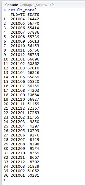
When we print out the final result...we will realize something that for sure, escaped our eyes before...


For 2010, the months start on April, meaning that from January to March there's no information...and the same happens to 2012 where the information end on April and from June to December there's nothing.

As we want to do a Forecasting using Neural Network...this incomplete data is never going to work...so we need to do something to fix it...

One thing to do at least for 2012, it's the Moving Average...which is basically grab the values from January to April, sum them, divide them by the number of months and then assign this value to May (201205)...then...grab the value from February to May and do the same thing for June...and so on -:)

For 2010 seems look a little bit more complicated...but it's almost the same...I used something that I like to call Backward Average...despite what the real name is -:P Basically, we grab the values from December to April, sum them, divide the value by the number of months and determine the value for March...and so on...

Let's see the code...

Moving and Backward Average
library("RODBC")

format_date<-function(p_date){
  p_date<-as.Date(as.character(p_date),"%Y%m%d")
  p_date<-format(p_date,"%Y%m")
  return(p_date)
}

moving_average<-function(p_values,year_start,month_start,year_end,month_end){
  month<-as.numeric(month_start) - 1
  init_month<-"01"
  if(length(month)==1){
    init_date<-paste(year_start,"0",month,sep='')
  }
  base_date<-paste(year_start,init_month,sep='')
  counter<-as.numeric(month_end) - as.numeric(month_start)
  
  values<-p_values
  
  for(i in 0:counter){
    values<-subset(values, FLDATE <= init_date & FLDATE >= base_date) 
    new_value<-floor(mean(values$SEATS))
    new_values<-data.frame(FLDATE=paste(year_start,month_start,sep=''),SEATS=new_value)
    p_values<-rbind(p_values,new_values)
    month_start<-as.numeric(month_start) + 1
    if(nchar(month_start)==1){
      month_start<-paste("0",month_start,sep='')
    }
    values<-rbind(values,new_values)
    month<-month + 1
    init_month<-as.numeric(init_month) + 1
    if(nchar(month)==1){
      init_date<-paste(year_start,"0",month,sep='')
    }else{
      init_date<-paste(year_start,month,sep='')
    }
    if(nchar(init_month)==1){
      base_date<-paste(year_start,"0",init_month,sep='')  
    }else{
      base_date<-paste(year_start,init_month,sep='')  
    }
  }
  return(p_values)
}

backward_average<-function(p_values,year_start,month_start,year_end,month_end){
  month<-as.numeric(month_start) - 1
  init_month<-"12"
  if(length(month)==1){
    init_date<-paste(year_start,"0",month,sep='')
  }
  base_date<-paste(year_start,init_month,sep='')
  counter<-as.numeric(month_start) - as.numeric(month_end)
  
  values<-p_values
  
  for(i in 0:counter){
    values<-subset(values, FLDATE <= base_date & FLDATE >= init_date) 
    new_value<-floor(mean(values$SEATS))
    new_values<-data.frame(FLDATE=paste(year_start,month_start,sep=''),SEATS=new_value)
    p_values<-rbind(p_values,new_values)
    month_start<-as.numeric(month_start) - 1
    if(nchar(month_start)==1){
      month_start<-paste("0",month_start,sep='')
    }
    values<-rbind(values,new_values)
    month<-month + 1
    init_month<-as.numeric(init_month) - 1
    if(nchar(month)==1){
      init_date<-paste(year_start,"0",month,sep='')
    }else{
      init_date<-paste(year_start,month,sep='')
    }
    if(nchar(init_month)==1){
      base_date<-paste(year_start,"0",init_month,sep='')  
    }else{
      base_date<-paste(year_start,init_month,sep='')  
    }
  }
  return(p_values)
}

ch<-odbcConnect("HANA",uid="SYSTEM",pwd="********")
result<-sqlQuery(ch,"SELECT FLDATE, SEATSOCC, SEATSOCC_B, SEATSOCC_F 
                 FROM SFLIGHT.SFLIGHT WHERE YEAR(FLDATE) BETWEEN '2010' AND '2012'")
odbcCloseAll()
dates<-result$FLDATE
dates<-format_date(dates)
result$FLDATE = dates
result_agg<-aggregate(cbind(SEATSOCC,SEATSOCC_B,SEATSOCC_F)~.,data=result,FUN=sum)
result_total<-data.frame(FLDATE=result_agg$FLDATE,SEATS=result_agg$SEATSOCC+
                         result_agg$SEATSOCC_B+result_agg$SEATSOCC_F,stringsAsFactors=FALSE)
result_total<-moving_average(result_total,"2012","05","2012","12")
result_total<-backward_average(result_total,"2010","03","2010","01")

When we run and execute this...we will see that in fact...we now have all the 3 years completed -;)


Now...we can finally use the Forecasting -;)

Neural_Network_Forecasting.R
library("RODBC")
library("forecast")

format_date<-function(p_date){
  p_date<-as.Date(as.character(p_date),"%Y%m%d")
  p_date<-format(p_date,"%Y%m")
  return(p_date)
}

moving_average<-function(p_values,year_start,month_start,year_end,month_end){
  month<-as.numeric(month_start) - 1
  init_month<-"01"
  if(length(month)==1){
    init_date<-paste(year_start,"0",month,sep='')
  }
  base_date<-paste(year_start,init_month,sep='')
  counter<-as.numeric(month_end) - as.numeric(month_start)
  
  values<-p_values
  
  for(i in 0:counter){
    values<-subset(values, FLDATE <= init_date & FLDATE >= base_date) 
    new_value<-floor(mean(values$SEATS))
    new_values<-data.frame(FLDATE=paste(year_start,month_start,sep=''),SEATS=new_value)
    p_values<-rbind(p_values,new_values)
    month_start<-as.numeric(month_start) + 1
    if(nchar(month_start)==1){
      month_start<-paste("0",month_start,sep='')
    }
    values<-rbind(values,new_values)
    month<-month + 1
    init_month<-as.numeric(init_month) + 1
    if(nchar(month)==1){
      init_date<-paste(year_start,"0",month,sep='')
    }else{
      init_date<-paste(year_start,month,sep='')
    }
    if(nchar(init_month)==1){
      base_date<-paste(year_start,"0",init_month,sep='')  
    }else{
      base_date<-paste(year_start,init_month,sep='')  
    }
  }
  return(p_values)
}

backward_average<-function(p_values,year_start,month_start,year_end,month_end){
  month<-as.numeric(month_start) - 1
  init_month<-"12"
  if(length(month)==1){
    init_date<-paste(year_start,"0",month,sep='')
  }
  base_date<-paste(year_start,init_month,sep='')
  counter<-as.numeric(month_start) - as.numeric(month_end)
  
  values<-p_values
  
  for(i in 0:counter){
    values<-subset(values, FLDATE <= base_date & FLDATE >= init_date) 
    new_value<-floor(mean(values$SEATS))
    new_values<-data.frame(FLDATE=paste(year_start,month_start,sep=''),SEATS=new_value)
    p_values<-rbind(p_values,new_values)
    month_start<-as.numeric(month_start) - 1
    if(nchar(month_start)==1){
      month_start<-paste("0",month_start,sep='')
    }
    values<-rbind(values,new_values)
    month<-month + 1
    init_month<-as.numeric(init_month) - 1
    if(nchar(month)==1){
      init_date<-paste(year_start,"0",month,sep='')
    }else{
      init_date<-paste(year_start,month,sep='')
    }
    if(nchar(init_month)==1){
      base_date<-paste(year_start,"0",init_month,sep='')  
    }else{
      base_date<-paste(year_start,init_month,sep='')  
    }
  }
  return(p_values)
}

ch<-odbcConnect("HANA",uid="SYSTEM",pwd="********")
result<-sqlQuery(ch,"SELECT FLDATE, SEATSOCC, SEATSOCC_B, SEATSOCC_F 
                 FROM SFLIGHT.SFLIGHT WHERE YEAR(FLDATE) BETWEEN '2010' AND '2012'")
odbcCloseAll()
dates<-result$FLDATE
dates<-format_date(dates)
result$FLDATE = dates
result_agg<-aggregate(cbind(SEATSOCC,SEATSOCC_B,SEATSOCC_F)~.,data=result,FUN=sum)
result_total<-data.frame(FLDATE=result_agg$FLDATE,SEATS=result_agg$SEATSOCC+
                         result_agg$SEATSOCC_B+result_agg$SEATSOCC_F,stringsAsFactors=FALSE)
result_total<-moving_average(result_total,"2012","05","2012","12")
result_total<-backward_average(result_total,"2010","03","2010","01")
result_total <- result_total[order(result_total$FLDATE),] 
result_ts<-ts(result_total$SEATS,frequency=12,start=c(2010,1))

fit <- nnetar(result_ts)
fcast <- forecast(fit)
plot(fcast)

Let's take a lot at the generated plot...


As we can see...the prediction for 2013 to 2015 is very low...but that's due to the fact that 2012 was a very low year...

Greetings,

Blag.

sábado, 27 de julio de 2013

SAP HANA OData and R

As you might have discovered by now...I love R...it's just an amazing programming language...

By now...I have integrate R and SAP HANA via ODBC and via the SAP HANA-R integration...but I have completely left out the SAP HANA OData capabilities.

For this blog, we're going to create a simple Attribute View, expose it via SAP HANA and then consume it on R to display a nice and fancy graphic -;)

First, let's create an Attribute View and call it FLIGHTS. This Attribute View is going to be composed of the tables SPFLI, SCARR and SFLIGHT and will output the fields PRICE, CURRENCY, CITYFROM, CITYTO, DISTANCE, CARRID and CARRNAME. If you wonder why so many fields? Just so I can use it in another examples -;)


With the Attribute View ready, we can create a project in the repository and the necessary files to expose it as an OData service.

First, we create the .xsapp file...which should be empty -:P

Then, we create the .xsaccess file with the following code...

.xsaccess
{
          "exposed" : true,
          "authentication" : [ { "method" : "Basic" } ]
}

Finally, we create a file called flights.xsodata

flights.xodata
service {
          "BlagStuff/FLIGHTS.attributeview" as "FLIGHTS" keys generate local "Id";
}

When everything is ready...we can call our service to test it...we can call it as either JSON or XML. For this example, we're going to call it as XML.


Now that we know its working...we can go and code with R -:D For this...we're going to need 3 packages (That you can install via RStudio or R itself), ggplot2, RCurl and XML.

HANA_OData_and_R.R
library("ggplot2")
library("RCurl")
library("XML")
web_page = getURL("XXX:8000/BlagStuff/flights.xsodata/FLIGHTS?$format=xml", userpwd = "SYSTEM:******")
doc <- xmlTreeParse(web_page, getDTD = F,useInternalNodes=T)
r <- xmlRoot(doc)
 
carrid<-list()
carrid_list<-list()
carrid_big_list<-list()
price<-list()
price_list<-list()
price_big_list<-list()
currency<-list()
currency_list<-list()
currency_big_list<-list()
 
for(i in 5:xmlSize(r)){
  carrid[1]<-xmlValue(r[[i]][[5]][[1]][[2]])
  carrid_list[i]<-carrid[1]
  price[1]<-xmlValue(r[[i]][[5]][[1]][[8]])
  price_list[i]<-price[1]
  currency[1]<-xmlValue(r[[i]][[5]][[1]][[7]])
  currency_list[i]<-currency[1] 
}
 
carrid_big_list<-unlist(carrid_list)
price_big_list<-unlist(price_list)
currency_big_list<-unlist(currency_list)
flights_table<-data.frame(CARRID=as.character(carrid_big_list),PRICE=as.numeric(price_big_list),
                          CURRENCY=as.character(currency_big_list))
flights_agg<-aggregate(PRICE~.,data=flights_table, FUN=sum)
flights_agg<-flights_agg[order(flights_agg$CARRID),]
 
flights_table<-data.frame(CARRID=as.character(flights_agg$CARRID),PRICE=as.character(flights_agg$PRICE),
                          CURRENCY=as.character(flights_agg$CURRENCY))
 
ggplot(flights_table, aes(x=CARRID, y=PRICE, fill=CURRENCY)) + geom_histogram(binwidth=.5, 
       position="dodge", stat="identity")

Basically, we're are reading the OData service that comes in XML format and parsing it into a tree so we can extract it's components. One thing that might call your attention is that we're using xmlValue(r[[i]][[5]][[1]][[2]]) where i starts from 5.

Well...there's an easy explanation -:) if we access our XML tree...the first value it's going to be "feed", the second "id" and so on...the fifth is going to be "entry" which is what we need. Then for the next [[5]]...inside "entry", the first value it's going to be "id", the second "title" and so on...the fifth is going to be "content" which is what we need. Then for the next [[1]]...inside "content", the first value it's going to be "properties" which is what we need. And for the last [[2]]...inside "properties" the first value it's going to be "id" and the second it's going to "carrid" which is what we need. BTW, xmlValue will get the value of the XML tag -:P

In other words...we need to analyze the XML schema and determine what we need to extract...after that, we simply need to assign those values to variables and create our data.frame.

Then we create an aggregation to sum the PRICE values (In other words, we're going to have the PRICE grouped by CARRID and CURRENCY), then we sort the values and finally we create a new data.frame so we can present the PRICE as character instead of numeric...just for better presentation of the graphic...

Finally...we call the plot and we're done -:)


Happy plotting! -:)

Greetings,

Blag.

jueves, 25 de julio de 2013

SAP HANA and R - Keep shining

Since I discovered Shiny and published my blog A Shiny example - SAP HANA, R and Shiny I always wanted to actually run a Shiny application from SAP HANA Studio, instead of having to call it from RStudio and having to use an ODBC connection.

A couple of days ago...this blog Let R Embrace Data Visualization in HANA Studio gave me the power I need to keep working on this...but of course...life is not that beautiful so I still need to do lots of things in order to get this done...

First...cygwin didn't worked for me -:(  so I used Xming instead -;)

Now...one thing that it's really important is to have all the X11 packages loaded into the R Server...so just do this...

Connect to your R Server via Putty and then type "yast" to enter the "Yet another setup tool". (Make sure you tick the X11 Forwarding)...


Search and install everything related to X11-Devel. Also install/update your Firefox browser (also on yast).


With that ready...we can keep going -;)

If you had R installed already...please delete it...as easy as this...

Deleting_R
rm -r R-2.15.0

Then, download the source again...keep in mind that we will need R-2.15.1

Get_R_Again
wget http://cran.r-project.org/src/base/R-2/R-2.15.1.tar.gz

Now...we need support for jpeg images...so let's download a couple of files...

Getting_support_for_images
wget http://prdownloads.sourceforge.net/libpng/libpng-1.6.3.tar.gz?download
wget http://www.ijg.org/files/jpegsrc.v9.tar.gz
 
tar zxf libpng-1.6.3.tar.gz
tar zxf jpegsrc.v9.tar.gz
 
mv libpng-1.6.3 R-2.15.1/src/gnuwin32/bitmap/libpng
mv jpeg-9 R-2.15.1/src/gnuwin32/bitmap/jpeg-9
 
cd R-2.15.1/src/gnuwin32/
cp MkRules.dist MkRules.local
vi MkRules.local

When you run vi on the file you should comment out the bitmap.dll source directory lines just like in the image (notice that I'm not dealing with TIFF images, as they didn't worked for me)...


Now, we need to into each folder and compile the libraries...

Compiling_libraries
cd R-2.15.1/src/gnuwin32/bitmap/libpng
./confire
make
make install
cd ..
cd jpeg-9
./configure
make
make install

When both libraries finished compiling...we can go an compile R -;)

Compiling_R
cd
cd R-2.15.1
./configure --enable-R-shlib --with-readline=no --with-x=yes
make clean
make
make install

As you can see...where using the parameter --with-x=yes to indicate that we want to have X11 into our R installation. As we compiled the JPEG and PNG libraries first...we will have support for this on R as well -;)

For sure...this will take a while...R compilation is a hard task -:P But in the end you should be able to confirm by doing this...

Checking_installation
R
capabilities()


Now...it's time to install Shiny -8)


Installing_Shiny
install.packages("shiny", dependencies=TRUE)

Easy as cake -:)

But here comes another tricky part...we need to create a new user...why? Because we mostly had a previous user to run the Rserve...that was created before we installed X11...so just create a new one -:)
Creating_new_user
useradd -m login_name
passwd login_name

For the X11 to work perfectly...we need to do another thing...

Get_Magic_Cookie
xauth list
echo $DISPLAY

This will return us a line that we should copy in a notepad...then...we need to log of and log in again via Putty (with the X11 Forwarding) but this time using our new user...the second line will tell us about the display, so copy that one as well...
Once logged with the new user...do this...

Assign_Magic_Cookie_and_Display
xauth add //Magic_Cookie_from_Notepad//
export DISPLAY=localhost:**.* //number get from the $DISPLAY...like 10.0 or 11.0

Now...we're are complete ready to go...

Start the Rserve server like this...

Start_Rserve
R CMD Rserve --RS-port 6311 --no-save --RS-encoding "utf8"

When our Rserve is up and running...it's time for SAP HANA to make it's entrance -;) What I really like about Shiny...is that...in the past you needed to create two files to make it work UI.R and Server.R...right now...Shiny uses the Bootstrap framework so we can create the webpage using just one file...or call it directly from the SAP HANA Studio -;)

Calling_Shiny_from_SAP_HANA_Studio.sql
CREATE TYPE SNVOICE AS TABLE(
CARRID CHAR(3),
FLDATE CHAR(8),
AMOUNT DECIMAL(15,2)
);
 
CREATE TYPE DUMMY AS TABLE(
ID INT
);
 
CREATE PROCEDURE GetShiny(IN t_snvoice SNVOICE, OUT t_dummy DUMMY)
LANGUAGE RLANG AS
BEGIN
library("shiny")
 
runApp(list(
  ui = bootstrapPage(
    pageWithSidebar(
      headerPanel("SAP HANA and R using Shiny"),
      sidebarPanel(selectInput("n","Select Year:",list("2010"="2010","2011"="2011","2012"="2012"))),
      mainPanel(plotOutput('plot', width="100%", height="800px"))
    )),
  server = function(input, output) {
    output$plot <- renderPlot({
      year<-paste("",input$n,sep='')
      t_snvoice$FLDATE<-format(as.Date(as.character(t_snvoice$FLDATE),"%Y%m%d"))
      snvoice<-subset(t_snvoice,format(as.Date(t_snvoice$FLDATE),"%Y") == year)
      snvoice_frame<-data.frame(CARRID=snvoice$CARRID,FLDATE=snvoice$FLDATE,AMOUNT=snvoice$AMOUNT)
      snvoice_agg<-aggregate(AMOUNT~CARRID,data=snvoice_frame,FUN=sum)
      pct<-round(snvoice_agg$AMOUNT/sum(snvoice_agg$AMOUNT)*100)
      labels<-paste(snvoice_agg$CARRID," ",pct,"%",sep="")
      pie(snvoice_agg$AMOUNT,labels=labels)
    })
  }
))
END;
 
CREATE PROCEDURE Call_Shiny()
LANGUAGE SQLSCRIPT AS
BEGIN
snvoice = SELECT CARRID, FLDATE, AMOUNT FROM SFLIGHT.SNVOICE WHERE CURRENCY = 'USD';
CALL GetShiny(:snvoice,DUMMY) WITH OVERVIEW;
END;
 
CALL Call_Shiny

I'm not going to explain the code, because you should learn some R and Shiny -:P But if you wonder why I have a "dummy" table...it's mainly because you can't create an Stored Procedure in R Lang that doesn't have an OUT parameter...so...does nothing but helps to run the code :)

When we call the script or the procedure Call_Shiny, the X11 from our Server is going to call Firefox which is going to appear on our desktop like this...


We can choose between 2010, 2011 and 2012...every time we choose a new value, the graphic will be automatically updated...


Before we finish...keep in mind that this approach is really slow...our R Server will send the information via X11 Forwarding to our machine, and will render the Firefox browser...also...we have a timer...so after so many seconds...we will have a Timeout...of course this can be configured, but for Performance purposes...we should limit the time the communication between our SAP HANA and R servers...

Hope you like this blog -:) and see you on the next one -;)

Greetings,

Blag.

jueves, 27 de junio de 2013

Schema Flexibility on SAP HANA - In a nutshell

Some time ago I post a blog called Getting flexible with SAP HANA that used SAP HANA, R and Twitter to demonstrate the Schema Flexibility capabilities...

I came to realize that even when that example is really cool...it's not really aimed for beginners, because you need a lot of R and Regular Expressions experience to fully understand what's going on...so...I decided to write a more simple blog...using only SAP HANA to show this awesome option...

So...what "Schema Flexibility" means? Well...it means that you can define a table with some columns and then dynamically add more columns at run time without the need of redefine the table structure...

First...let's create a table using plain SQL...

Create Table
CREATE COLUMN TABLE Products(
PRODUCT_CODE VARCHAR(3),
PRODUCT_NAME NVARCHAR(20),
PRICE DECIMAL(5,2)
) WITH SCHEMA FLEXIBILITY;

As you can see...it's just a table...but we're adding the WITH SCHEMA FLEXIBILITY option...

Now...we can simply insert one product...

Insert Product
INSERT INTO Products values ('001','Blag Stuff', 100.99);

Let's say that we need to add a new product...that comes in different colors...but our table doesn't have a COLOR column defined...but it doesn't matter...our table is flexible enough to hold it up...

Insert New Product
INSERT INTO Products (PRODUCT_CODE,PRODUCT_NAME,PRICE,COLOR) values ('002','More Blag Stuff',100.99,'Black');

Notice that we're defining all the columns and adding a new one called "COLOR"...and simply pass the new value...when we select all the records from the table, we will have this...


As you can see...for the second record, we have the new column "COLOR" along with it's value...for the first record, we simple have an "?" because the "COLOR
column didn't exist at the time of it's creation...

Now...let's say we need to add another new product...that doesn't come in colors...

Insert last new product
INSERT INTO Products (PRODUCT_CODE, PRODUCT_NAME, PRICE) values ('003','Even More Blag Stuff',101.99);

Notice that we need to specify the "regular" column names, but we don't need to care about the dynamic column...ll have this when getting all records...


As the column "COLOR" already exist at the time of the creation of the last product...we will see a "?"  value again...

I hope that with this small blog...this gets more clear -:) Even where there are not so many use cases for this...I expect many people to get creative and use this cool feature...

Small update

You might have realized that when you create a new column..it's going to be generated as NVARCHAR(5000)...so that's not very helpful right?

Sadly...we cannot change this because the feature is not "yet" supported...and that's because the field length can't be shortened...

However, if we are passing a numeric value...then we're allow to change it...consider the following example...

Altering COLOR Column
INSERT INTO Products values ('001','Blag Stuff', 100.99);
 
INSERT INTO Products (PRODUCT_CODE,PRODUCT_NAME,PRICE,QUANTITY) values ('002','More Blag Stuff',100.99,10);
 
ALTER TABLE Products ALTER (QUANTITY INT);

Here...we're adding a new column called "QUANTITY" with a value of 10...at first is going to be created a NVARCHAR(5000) but with a simple ALTER TABLE we can change it to INT...

Now, let's say we need to update the first field to include a quantity as well...using a simple UPDATE will do the trick...

Updating a field
UPDATE Products
SET QUANTITY = 20
WHERE PRODUCT_CODE = '001';


Greetings,

Blag.

jueves, 30 de mayo de 2013

AngularJS, PHP and SAP HANA

Yesterday, I realized that it's been a while since a post a blog about SAP HANA...so I decided to think about something cool to write about...checking my feeds, I came to notice AngularJS The Super Heroic JavaScript MVW Framework...

So...what is good about AngularJS? Well...according to them...

Other frameworks deal with HTML’s shortcomings by either abstracting away HTML, CSS, and/or JavaScript or by providing an imperative way for manipulating the DOM. Neither of these address the root problem that HTML was not designed for dynamic views.

So...in this blog, we're going to use PHP to get information from SAP HANA, return them as a JSON object and be presented by AngularJS.

Let's get our hands dirty -;)

First...I create a System DSN for my SAP HANA connection...so I could call it from PHP...

menu.php
<?php
$conn = odbc_connect("HANA_SYS","SYSTEM","********", SQL_CUR_USE_ODBC);
$query = "SELECT table_name from SYS.CS_TABLES_ where schema_name = 'SFLIGHT'";
$rs = odbc_exec($conn,$query);
$result = array();
while($row = odbc_fetch_array($rs)){
          $menu["table_name"] = $row["TABLE_NAME"];
          array_push($result,$menu);
}
echo json_encode($result);
?>

This code will allow us to get all the tables names included in the SFLIGHT schema...so we can present a dropdown list to choose from...

tables.php
<?php
$data = file_get_contents("php://input");
$objData = json_decode($data);
$data = $objData->data;
$conn = odbc_connect("HANA_SYS","SYSTEM","*********", SQL_CUR_USE_ODBC);
$query = "select column_name from SYS.CS_COLUMNS_ A inner join SYS.CS_TABLES_ B";
$query .= " on A.table_oid = B.table_oid where schema_name = 'SFLIGHT'";
$query .= " and table_name = '$data' and internal_column_id > 200 order by internal_column_id";
$rs = odbc_exec($conn,$query);
$result = array();
$fields = array();
$fields_array = array();
while($row = odbc_fetch_array($rs)){
          array_push($result,$row["COLUMN_NAME"]);
          $fields["FIELDS"] = $row["COLUMN_NAME"];
          array_push($fields_array,$fields);
}
sort($fields_array);
 
 
$content = array();
$table = array();
$query = "select * from SFLIGHT.$data";
$rs = odbc_exec($conn,$query);
array_push($content,$fields_array);
while($row = odbc_fetch_array($rs)){
          for($i=0;$i<count($result);$i++){
                    $table["$result[$i]"] = $row["$result[$i]"];
          }
          array_push($content,$table);
}
echo json_encode($content);
?>

This code will get a table name as parameter and will get the Fields name and the contents of the table...both PHP scripts will return a JSON object...

get_menu.js
function MenuCtrl($scope, $http) {
    $scope.url = 'menu.php';
        
        $http.post($scope.url).
        success(function(data, status) {
            $scope.status = status;
            $scope.data = data;
            $scope.tables = data;
        })
        .
        error(function(data, status) {
            $scope.data = data || "Request failed";
            $scope.status = status;        
        });
 
            $scope.gettable = function() {
                      $scope.url = 'tables.php';
        $http.post($scope.url, { "data" : $scope.table}).
        success(function(data, status) {
            $scope.status = status;
            $scope.data = data;
                              $scope.contents = data;
        })
        .
        error(function(data, status) {
            $scope.data = data || "Request failed";
            $scope.status = status;        
        });
    };
}

This code will simply read back the JSON objects generated by the PHP scripts...the first part for dropdown list and the second for the tables fields and contents...

Finally...we have our HTML which call the AngularJS script to perform the magic...

main.html
<!DOCTYPE html>
<html ng-app>
<head>
<title>Angular.JS, PHP and SAP HANA</title>
    <link rel="stylesheet" href="css/bootstrap.min.css" type="text/css" />
    <script src="http://code.angularjs.org/angular-1.0.0.min.js"></script>
    <script src="get_menu.js"></script>
</head>
<body ng-controller='MenuCtrl'>
<div align="center">
          <H1>AngularJS, PHP and SAP HANA</H1>
          <form>
                    <label>Choose table:</label>
                    <select ng-model="table">
                              <option ng-repeat="table in tables" value='{{table.table_name}}'>{{table.table_name}}
                    </select>
                    <button type="submit" class="btn" ng-click="gettable()">Get Table</button>
          </form>
          <br/>
          <table border="1" ng-show="contents.length">
                    <tr ng-repeat="(key, value) in contents" ng-show="$first">
                              <th ng-repeat="values in value")>{{values.FIELDS}}</th>
                    </tr>
                    <tr ng-repeat="(key, value) in contents" ng-show="!$first">
                              <td ng-repeat="values in value")>{{values}}</td>
                    </tr>
          </table>
</div>
</body>
</html>

This code is simple...it will grab the JSON objects and simply use repeaters to read the information and place it on both the menu and the table.

Here's are some screenshots of the application running...


Now...you might notice that the fields are actually sorted! And not in the defined order...well...this is a JavaScript problem more than an AngularJS problem...at least that's what I found out...but...who cares in the end...the data is presented and that's all that matters -;)

One thing to notice as well...is that AngularJS is not particularly fast...for some big tables...it will throw up a time limit exception...even when SAP HANA will send back the information really fast...and for sure PHP is going to create the JSON objects as fast as well...I guess the root problem is that AngularJS will sort the columns, read each line and then construct the table...or...maybe it's just because I'm an AngularJS newbie -:P

Either way...this my was my first experience ever with AngularJS...and I gotta say...I had a lot of fun! -:D The learning curve is really fast and AngularJS provide many cool features that makes it and really good alternative for web development -;)

See you in my next blog -}:)

Greetings,

Blag.

martes, 23 de abril de 2013

PhoneGap 2.x Mobile Application Development Hotshot - Book Review

As I announced early on my post On my book shelve - PhoneGap 2.x Mobile Application Development Hotshot, I was reading this book...and now...I'm ready to write a review about it.


First thing first...I read it...but didn't actually spend too much time doing all the projects, so I'm for sure will read it again -:D

So...is this book good or bad? I will say...it's really good!

For me...the best way to learn a new programming language or tool...is by actually build stuff with it...and this book is full of practical projects that will dive you deep in the PhoneGap development.

The book include projects that deal with Twitter, Camera, Storage and even GeoLocation...also...it includes a small game! How awesome is that?! Really awesome -:)

The projects are easy to follow, but of course...they are not simple...they are complex and that adds more flavor to them...you really need to be focused on what you're doing to get the full grasp of it...but again...by doing it yourself, you will learn it more quickly and will not forget it anytime soon...

I want to show you a couple of images of two of the projects included in the book...so you can have an idea of what you're going to build...


BTW...even when I'm posting only Android based images...the book focuses on both IOS and Android.

If you have never used PhoneGap before...or you're a newbie with little experience like me...then this book really is for you...happy coding!

Greetings,

Blag.

martes, 16 de abril de 2013

On my book shelve - PhoneGap 2.x Mobile Application Development Hotshot

I'm always reading new programming books, so I guess it's good to alert people that I'm reading something and that I'm planning to write a review so they can know if the book its good or not...

This new section is going to be called "On my book shelve" and I want to start with the book called:

PhoneGap 2.x Mobile Application Development Hotshot

I have tried PhoneGap once, when I wrote about its integration with SAP HANA -:)

This books really looks good as it covers a lot of Projects that in my humble opinion...its the best way to learn programming...by actually coding -;)

I will read the book and let you know my thoughts -:)

Greetings,

Blag.


miércoles, 10 de abril de 2013

A new beginning...

After 3 years living in Montreal, Canada...with 1 years and 8 months with Beyond Technologies and 1 year and 3 months with SAP Labs Canada...I'm making my bags again...

This time, I'm moving along with my family to California...where I will work for SAP Labs in Palo Alto.

Why are we moving? Simply put...my team Developer Experience is divided between Palo Alto and Waldorf...being me and my team mate Vitaliy Rudnyskiy and I the only ones on our countries (Him in Poland and me in Canada)...that's why it makes perfect sense to go where the team is -;) (I wasn't of course willing to learn German).

I'm flying this Saturday, so my last days in Montreal are already here...while I worked from home most of the time, the times I visit the office were amazingly good...I made some really good friends like Pakdi, Jon, Elsa, Krista, Pierre and Nolwen. I will keep in touch with them of course -:)

As I'm moving to the Palo Alto office...both my title Development Expert and my duties will remain the same...well...actually...my duties are going to increase -:P But who cares...I love my job so much that all new duties are welcome -;)

One of the really good things about this move is that I will be able to attend all the cool meeting, hackatons and gatherings that happen in the US...so I'm really looking for that...

Of course...after all the craziness of the relocation is over...I will continue blogging like crazy, trying to give you the best coding experiences -:)

Greetings,

Blag.