Prediction model with HANA and R

These days, I have been reading and playing a lot with R, and I really come to love it...of course, I don't have a clue on those weird statistics formulas, but it doesn't mean I can't use R and try do some awesome stuff with it.

So, yesterday I was thinking about doing another integration between HANA and R, my new adopted kids, so I came with the idea of building a prediction model for a flight company. I followed this steps.

1.- First, I need to choose a table, so I picked SNVOICE:

This table offers us, the carrier id, the date and book id, meaning the amount of tickets sold in a particular day. And from here when can do some calculation and determine how many tickets were sold in each month of a particular year.

2.- I needed a table to store my new information, so I created the table TICKETS_BY_YEAR:

3.- I needed a Procedure script to analyse the table, determine the total amount per day of the month and then gave a grand total per month.

CREATE PROCEDURE GetTicketsByMonth 
(IN var_year NVARCHAR(4),IN var_carrid NVARCHAR(2))
LANGUAGE SQLSCRIPT AS
v_found NVARCHAR(2) := 1;
sum_bookid INT;
v_date NVARCHAR(8) := '';
BEGIN                
TT_MONTH = select fldate, count(bookid) as "BOOKID"
           from sflight.snvoice 
           where year(fldate) = VAR_YEAR and carrid = VAR_CARRID
           group by fldate
           order by fldate asc;
v_date := (:var_year * 10000) + 101;
while :v_found <= 12 do 
select sum(bookid) into sum_bookid
from :TT_MONTH
where month(fldate) = :v_found;
insert into TICKETS_BY_YEAR
values(v_date,sum_bookid);
v_date := :v_date + 100;
v_found := :v_found + 1;
end while;           
END;

4.- Of course...I needed to call my Procedure...

CALL P075400.GetTicketsByMonth('2011','''AA''');

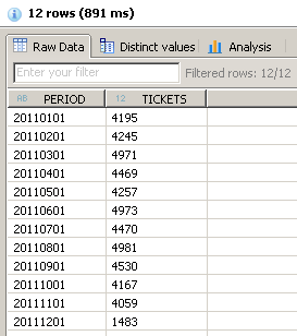
5.- Once finished, I checked my table to see if everything worked as expected...

6.- After realizing that my data was nice and clean, I exported to an .CSV file (Sorry...no pics this time...I already post it in a previous blog)

7.- I went to my R Studio and start coding...

Flight_Tickets=read.csv(file="Flight_Tickets.csv",header=TRUE)
period=Flight_Tickets$PERIOD
tickets=Flight_Tickets$TICKETS
var_year=substr(period[1],1,4)
var_year=as.integer(var_year)
var_year=var_year+1
var_year=as.character(var_year)
new_period=gsub("^\\d{4}",var_year,period)
next_year=data.frame(year=new_period,StringsAsFactors=FALSE)
prt.lm=lm(tickets ~ period)
pred=predict(prt.lm,next_year,interval="none")

plot(tickets,type="b",
     col="red",
     main="Annual Tickets Sale",
     xlab="Months",ylab="Tickets")
lines(pred,type="b",col="blue")
legend("bottomleft",inset=.05,title="Real vs. Predicted",
       c("Real","Predicted"),
       lty=c(1,1),col=c("red","blue"))

8.- I watch my generated graphic showing the real tickets sale vs. the predicted tickets sale. The real is for every month of 2011 and the predicted for every month of 2012.

9.- Nothing to do here...it's done -:)

10.- See you next time with more HANA, R or another nice technology.

Greetings,

Blag.